English only
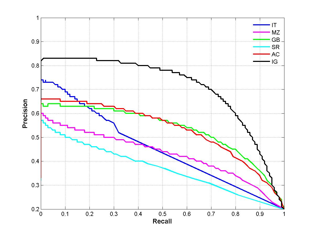
Detection of visually salient image regions is useful for applications like object segmentation, adaptive compression, and object recognition. In this paper, we introduce a method for salient region detection that outputs full resolution saliency maps with well-defined boundaries of salient objects. These boundaries are preserved by retaining substantially more frequency content from the original image than other existing techniques. Our method exploits features of color and luminance, is simple to implement, and is computationally efficient. We compare our algorithm to five state-of-the-art salient region detection methods with a frequency domain analysis, ground truth, and a salient object segmentation application. Our method outperforms the five algorithms both on the ground truth evaluation and on the segmentation task by achieving both higher precision and better recall.
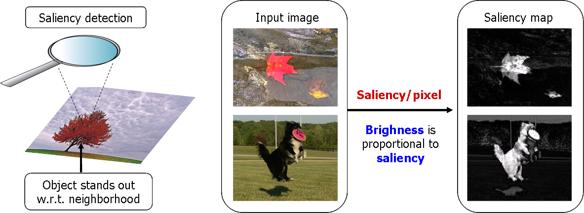
Salient regions and objects stand-out with respect to their neighborhood. The goal of our work was to compute the degree of standing out or saliency of each pixel with respect to its neighbourhood in terms of its color and lightness properties. Most saliency detection methods take a similar center-versus-surround approach. One of the key decisions to make is the size of the neighborhood used for computing saliency. In our case we use the entire image as the neighborhood. This allows us to exploit more spatial frequencies than state-of-the-art methods (please refer to the paper for details) resulting in uniformly highlighted salient regions with well-defined borders.
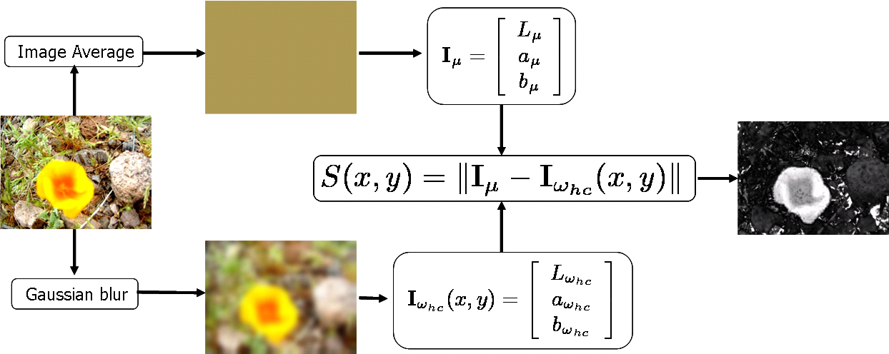
In simple words, our method find the Euclidean distance between the Lab pixel vector in a Gaussian filtered image with the average Lab vector for the input image. This is illustrated in the figure below. The URL's provided right below the image provide a comparison of our method with state-of-the-art methods.
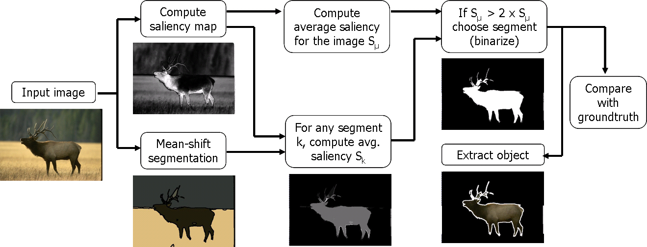
The salient region segmentation algorithm illustrated below is a modified version of the one presented in [5]. There are two differences with respect to the previous algorith: instead of k-means segmentation mean-shift segmentation is used, and the threshold for choosing salient regions is adaptive (to the average saliency of the input image).
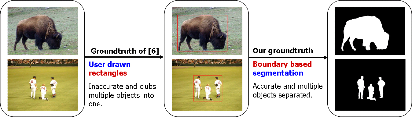
We derive a ground truth database of 1000 image from the one presented in [6]. The ground truth in [6] is user-drawn rectangles around salient regions. This is inaccurate and clubs multiple objects into one. We manually-segment the salient object(s) within the user-drawn rectangle to obtain binary masks as shown below. Such masks are both accurate and allows us to deal with multiple salient objects distinctly. The ground truth database can be downloaded from the URL provided below the illustration.
[1] L. Itti, C. Koch, and E. Niebur. A model of saliency-based visual attention for rapid scene analysis. PAMI 1998.
[2] Y.-F. Ma and H.-J. Zhang. Contrast-based image attention analysis by using fuzzy growing. ACM MM 2003.
[3] J. Harel, C. Koch, and P. Perona. Graph-based visual saliency. NIPS 2007.
[4] X. Hou and L. Zhang. Saliency detection: A spectral residual approach. CVPR 2007.
[5] R. Achanta, F. Estrada, P. Wils, and S. Süsstrunk. Salient region detection and segmentation. ICVS 2008.
[6] Z. Wang and B. Li. A two-stage approach to saliency detection in images. ICASSP 2008.
This work is in part supported by the National Competence Center in Research on Mobile Information and Communication Systems (NCCR-MICS), a center supported by the Swiss National Science Foundation under grant number 5005-67322, the European Commission under contract FP6-027026 (K-Space), and the PHAROS project funded by the European Commission under the 6th Framework Programme (IST Contract No. 045035).
The precision-recall curve presented in the paper (Figure 5) was for the first 500 images. The figure for 1000 images that should have been in the paper is shown below. The color conversion function was reimplemented. It shows our method to be doing better than in the figure in the paper. One can reproduce this curve using the C++ code provided for download on this page. Also, Tf values indicated on in Figure 5 can be misleading. Please note that the precision and recall values for a given threshold do not necessarily fall on a vertical line for each of the curves. So in the figure below we are doing away with Tf.